The MCMC Inference Engine Behind a PPL

Have you ever used a Probabilistic Programming Language (PPL) like PyMC or Stan and wondered what happens inside when you write pm.sample()?

In this tutorial, we’ll pull back the curtain. Instead of building a full-fledged language, we’re going to do something more fundamental: build the simple MCMC engine that lies at the heart of a PPL.

The Problem: Our Inaccurate Thermometer

Let’s say we have five temperature readings from a cheap thermometer. Traditionally, we manually calculate sample mean, standard deviation, get confidence intervals, etc.

Our goal is to estimate the true temperature of the room, not as a single number, but as a distribution of plausible values.

measurements = [22.1, 21.8, 22.3, 21.9, 22.0]
estimated_temp = sum(measurements) / len(measurements)  #22.02°C
estimated_temp

22.02

But this doesn’t tell us anything about our uncertainty. Is the true temperature exactly 22.02°C? Or is it likely to be somewhere between 21.9°C and 22.1°C?

That’s where PPLs come in. They are powerful tools that let you build models of your beliefs about a problem and then use data to refine those beliefs. Instead of you doing the heavy lifting of statistical formulas, the PPL does it for you.

The PPL Approach: Modeling Beliefs

With a PPL, we state our beliefs (or assumptions) as probability distributions:

Prior Belief about Temperature: We think the true temperature is probably around 21°C. We model this with a Normal distribution. This is our prior.

Prior Belief about Error: We know the thermometer has some positive measurement error. We model this with a Half-Normal distribution.

Likelihood of the Data: Each reading is the true temperature plus some of that random error. This connection between parameters and data is our likelihood.

Minor note: The word “belief” has some historical baggage. I’m really talking about mathematical representations of uncertainty that must be explicitly stated and can be tested.

Here is how a popular PPL (PyMC) would handle it:

import pymc as pm
import numpy as np

with pm.Model() as professional_model:
    true_temp = pm.Normal("true_temp", mu=21, sigma=2)
    error = pm.HalfNormal("error", sigma=0.5)
    readings = pm.Normal("readings", mu=true_temp, sigma=error, observed=measurements)

    # This one line runs a highly sophisticated MCMC engine (NUTS)
    trace = pm.sample(1000)

Or in more mathematical terms:

with Model() as my_model:
    μ = sample("mu", Normal(0, 1))
    σ = sample("sigma", HalfNormal(1))
    for i in range(N):
        x_i = sample(f"x_{i}", Normal(μ, σ))
        observe(f"obs_{i}", x_i, data[i])

By defining the model this way, the PPL can then run powerful inference algorithms (like MCMC, NUTS, etc.) to figure out the most plausible values for true_temp and measurement_error, given our observed readings.

The Inference Engine

The job of an inference engine is to take two inputs:

• The Model: Your description of priors and the likelihood.

• The Data: Your observed measurements.

And produce one output:

• The Posterior Distribution: The updated, data-informed beliefs about your parameters (true_temp and error).

There are many ways to build an engine (e.g., Variational Inference, MCMC, SMC, HMC, etc.). We will build ours using Markov Chain Monte Carlo (MCMC) because it is fundamental to understanding how modern Bayesian inference works.

Before we write any code, let’s understand the logic our engine will follow.

Imagine the probability of any combination of parameters (true_temp and error) as a landscape. The higher the probability, the better that combination explains our data. This landscape is called the posterior probability surface. Our goal is to create a map of this landscape, especially its highest peaks.

Since we can’t see the whole map at once, our MCMC engine will work like an explorer tasked with mapping this terrain in the dark. The specific set of rules our explorer will follow is called the Metropolis-Hastings algorithm (explained later).

Note: For more resources on MCMC, check out this video for a quick introduction or this for a deep dive

Now that we understand the logic, let’s translate that process into Python code

import numpy as np
import scipy.stats as stats
import matplotlib.pyplot as plt
import arviz as az

class SimPPL:
    """A minimal PPL engine using Metropolis-Hastings MCMC."""

    def __init__(self, model_func):
        self.model_func = model_func
        self.param_info = {}

    def sample(self, name, dist, **kwargs):
        """Our language's 'verb' for defining a parameter and its prior."""
        self.param_info[name] = {'dist': dist, 'args': kwargs}

    def log_prior(self, params):
        """Calculates the log probability of the parameters (our prior belief)."""
        log_p = 0
        for name, value in params.items():
            info = self.param_info[name]
            log_p += info['dist'](**info['args']).logpdf(value)
        return log_p

    def log_likelihood(self, params, data):
        """Calculates the log probability of the data given the parameters."""
        mu = params['true_temp']
        sigma = params['error']
        if sigma <= 0: return -np.inf # Cannot have negative or zero error
        return np.sum(stats.norm.logpdf(data, loc=mu, scale=sigma))

    def run(self, data, n_chains=1, num_samples=5000, burn_in=1000):
        """Runs the MCMC inference engine."""
        all_traces = []
        for _ in range(n_chains):
            trace = {name: [] for name in self.param_info.keys()}

            # Rule 1: Start at a random point
            current_params = {name: info['dist'](**info['args']).rvs() for name, info in self.param_info.items()}
            if 'error' in current_params and current_params['error'] <= 0:
                current_params['error'] = 0.1

            current_log_posterior = self.log_likelihood(current_params, data) + self.log_prior(current_params)

            # Rule 5: Repeat thousands of times
            for i in range(num_samples):
                # Rule 2: Propose a new step
                proposed_params = current_params.copy()
                for name in proposed_params:
                    proposed_params[name] += np.random.normal(0, 0.1)

                # Rule 3: Evaluate the new step
                proposed_log_posterior = self.log_likelihood(proposed_params, data) + self.log_prior(proposed_params)

                # Rule 4: Accept or reject
                acceptance_ratio = np.exp(proposed_log_posterior - current_log_posterior)
                if np.random.rand() < acceptance_ratio:
                    current_params = proposed_params
                    current_log_posterior = proposed_log_posterior

                # Rule 5: Record the position (after a "burn-in" warm-up period)
                if i >= burn_in:
                    for name, value in current_params.items():
                        trace[name].append(value)

            all_traces.append(trace)

        print(f"Inference complete for {n_chains} chain(s).")
        return all_traces

Let’s break down the SimplePPL class we just built. Each method has a specific job in translating our conceptual MCMC rules into working Python code.

__init__(self, model_func)

A constructor to set up our PPL instance. It takes a user-defined function, model_func, which will describe the statistical model we want to analyze. It also initializes a dictionary, param_info, which will store the definitions of our model’s parameters (i.e., our priors). Note that the trace (our results) is not created here; it will be generated by the run method for each independent chain.

sample(self, name, dist, **kwargs)

This is how we define a parameter in our model. It records the name of the parameter (e.g., 'true_temp'), its prior distribution (e.g., stats.norm), and the distribution’s arguments (e.g., loc=21, scale=2). This information is crucial for the MCMC algorithm to know what constitutes a “believable” parameter value when calculating the prior probability.

In our example, we will call this twice:

• ppl_instance.sample('true_temp', stats.norm, ...) declares our belief that the true temperature follows a Normal distribution.
• ppl_instance.sample('error', stats.halfnorm, ...) declares our belief that the measurement error follows a Half-Normal distribution.

log_prior(self, params)

This method calculates how probable a given set of parameter values is, according to the priors we defined with sample. It computes the logarithm of the prior probability (we use logs for numerical stability and easier math).

During the MCMC run, if the algorithm wants to test the combination {'true_temp': 21.5, 'error': 0.4}, this method will calculate log(P(true_temp=21.5)) + log(P(error=0.4)) using the Normal and Half-Normal distributions we specified.

log_likelihood(self, params, data)

This is the core of the observation step. It calculates how likely our observed data is, given a specific set of parameters. This is the likelihood.

In our example, this method answers the question: “If the true temperature were 22.1 and the error were 0.5, what’s the probability we would have seen our actual measurements of [22.1, 21.8, ...]?” The MCMC algorithm uses this likelihood to favor parameters that better explain the data we actually saw.

run(self, data, n_chains=1, ...)

This method is the engine of our PPL. It implements the Metropolis-Hastings MCMC algorithm and now supports running multiple independent chains to help us check for convergence.

For each chain requested by n_chains, the engine performs the following steps:

• Initialize: It starts at a random point in the parameter space, with values for true_temp and error drawn from their priors. This is “Rule 1” from our intuitive explanation.

• Propose a New Point: It iteratively moves the current parameter values slightly to propose a new candidate point. This simple random walk is our proposal mechanism.

• Evaluate the New Point: It calculates how “good” this new point is by combining the log_prior (is the new point believable?) and the log_likelihood (does it explain the data well?). This combination gives the log_posterior.

• Accept or Reject: It computes the ratio of the new point’s posterior probability to the old one’s. Based on this ratio, it probabilistically decides whether to move to the new point or stay put. This is the core Metropolis-Hastings step.

• Store the Sample: After an initial “burn-in” period (to let the algorithm settle), it begins recording the current accepted parameter values at each step. These recorded values form a single trace.

Finally, after running this process for each chain, the method returns all_traces, which is a list containing the individual trace from each independent run.

Let’s use our class to solve the thermometer problem

# 1. Define the model using our PPL's "language"
def temperature_model(ppl_instance):
    ppl_instance.sample('true_temp', stats.norm, loc=21, scale=2)
    ppl_instance.sample('error', stats.halfnorm, loc=0, scale=0.5)

# 2. Set up the data and the engine
measurements = np.array([22.1, 21.8, 22.3, 21.9, 22.0])
model = SimPPL(model_func=temperature_model)
model.model_func(model) # Initialize the parameters

# 3. Run the inference (we'll start with one chain)
traces = model.run(data=measurements, n_chains=1, num_samples=10000)
single_trace = traces[0]

# 4. Analyze the results
az_trace = az.from_dict(single_trace)
az.plot_posterior(az_trace, round_to=3)
plt.show()

Inference complete for 1 chain(s).

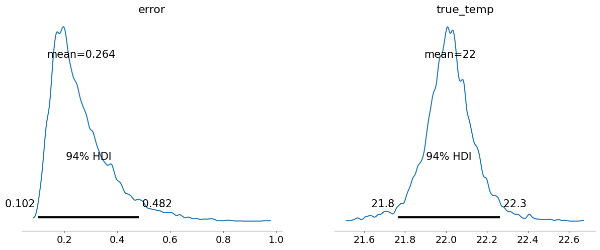
The true_temp chart shows our model’s updated belief about the temperature. It’s centered around 22.0°C, but the width of the distribution shows our uncertainty.

The 94% HDI (Highest Density Interval) gives us a credible interval. We can be 94% confident that the true temperature lies within this range.

The error chart shows the plausible values for the thermometer’s standard deviation of error.

Where does our Engine Struggle?

Our engine provides one theoretical guarantee: asymptotic convergence (The distribution of the samples generated by the MCMC chain will become an increasingly better approximation of the true posterior distribution as the number of steps in the chain approaches infinity).

But… no practical ones (since practically we cannot run infinite samples). By testing its limits, we can understand why professional PPLs are so powerful and how can we improve our inference engine to provide more guarantees.

Guarantees: Convergence Check

Did our MCMC chain run long enough? We can check by running multiple chains from different starting points to see if they converge to the same place.

# Run the model again, this time with 4 chains
multi_traces = model.run(data=measurements, n_chains=4, num_samples=5000)

# Visualize the trace paths
fig, (ax1, ax2) = plt.subplots(2, 1, figsize=(12, 6), sharex=True)
colors = ['r', 'g', 'b', 'k']
for i, trace in enumerate(multi_traces):
    ax1.plot(trace['true_temp'], color=colors[i], alpha=0.7)
    ax2.plot(trace['error'], color=colors[i], alpha=0.7)

ax1.set_title('Trace Plot: Did the Chains Converge?')
ax1.set_ylabel('true_temp')
ax2.set_ylabel('error')
ax2.set_xlabel('MCMC Step')
plt.show()

Inference complete for 4 chain(s).

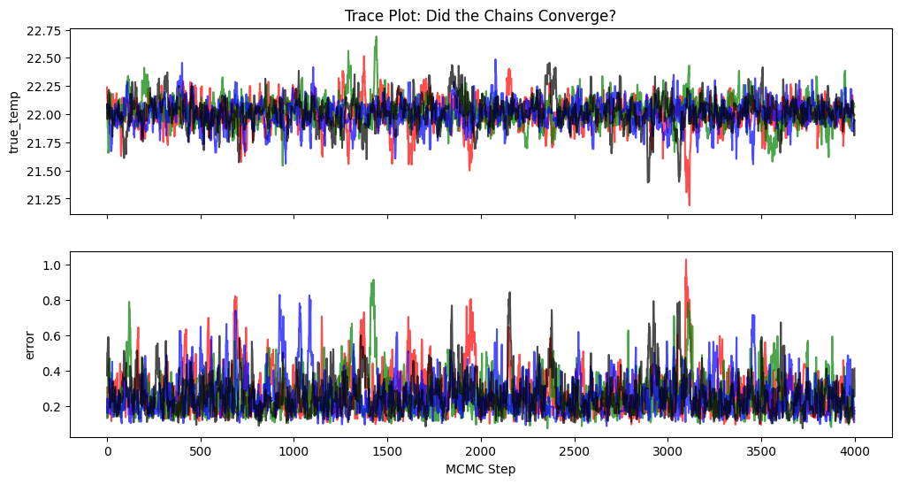
The chains are all exploring the same distribution so this gives us confidence that for this simple problem, our sampler has likely converged.

Guarantees: Efficiency Check

How effectively does our sampler explore the space? We can check with an autocorrelation plot. High correlation means the sampler is inefficient.

az.plot_autocorr(az.from_dict(single_trace))
plt.show()

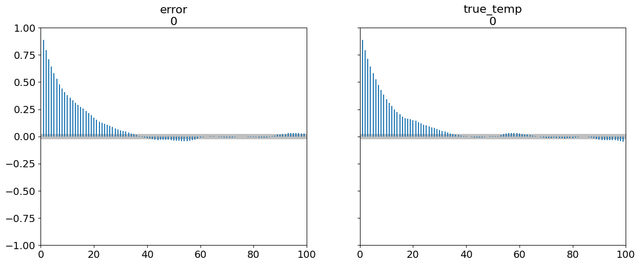
The correlation (y-axis) dies off very slowly over many lags (x-axis). This is a classic sign of an inefficient random-walk sampler. Each sample is highly dependent on the previous one. A professional sampler like NUTS would show this correlation dropping to near-zero almost immediately.

The Simplest Problem Where It All Breaks Down

Our simple engine works for our simple problem. But where does it completely fail?

The Problem: Inferring two parameters that are highly correlated.

This creates a long, narrow region in the probability space that our random-walk sampler is too weak to explore.

# 1. Define a problem with correlated parameters
true_mean = [0, 0]
true_cov = [[1.0, 0.98], [0.98, 1.0]] # Very high correlation
data_corr = np.random.multivariate_normal(true_mean, true_cov, 100)

# 2. Define the model and a new likelihood
def correlated_model(ppl_instance):
    ppl_instance.sample('x', stats.norm, loc=0, scale=5)
    ppl_instance.sample('y', stats.norm, loc=0, scale=5)

def log_likelihood_corr(params, data):
    return np.sum(stats.multivariate_normal.logpdf(data, mean=[params['x'], params['y']], cov=true_cov))

# 3. Run the engine
model_corr = SimPPL(model_func=correlated_model)
model_corr.log_likelihood = log_likelihood_corr
model_corr.model_func(model_corr)
trace_corr = model_corr.run(data=data_corr, n_chains=1, num_samples=5000)[0]

# 4. Visualize the failure
x_grid, y_grid = np.mgrid[-4:4:.1, -4:4:.1]
pos = np.dstack((x_grid, y_grid))
z = stats.multivariate_normal(true_mean, true_cov).pdf(pos)

fig, (ax1, ax2) = plt.subplots(1, 2, figsize=(12, 5))
ax1.contourf(x_grid, y_grid, z, cmap='viridis')
ax1.plot(trace_corr['x'], trace_corr['y'], 'r-', alpha=0.3, label='Sampler Path')
ax1.set_title("Inference Failure: Sampler cannot explore the 'canyon'")
ax1.legend()

ax2.plot(trace_corr['x'])
ax2.set_title("Resulting Bad Trace Plot")
plt.show()

<ipython-input-6-1993481708>:56: RuntimeWarning: overflow encountered in exp
  acceptance_ratio = np.exp(proposed_log_posterior - current_log_posterior)

Inference complete for 1 chain(s).

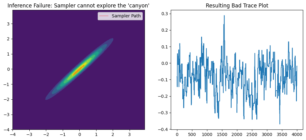
The result is a total failure

Instead of a smooth collection of points that maps out the entire yellow canyon, our samples are clustered in disconnected blobs. The sampler is clearly not exploring the space freely. It gets stuck in one small area of the canyon for a long time, then makes a large, inefficient jump to another area, completely missing the regions in between.

You can see in the trace plot, sections where the line stays at the same level for many steps. This is the visual evidence of the sampler being stuck. During these times, it is constantly proposing bad moves (stepping off the “canyon ridge”) and rejecting them, so its position doesn’t change. Then, the flat sections are punctuated by large vertical jumps. This is when the sampler finally gets lucky with a proposal that is accepted, allowing it to “jump” from one blob on the 2D plot to another.

How is this problem solved? NUTS!

The reason NUTS succeeds where our simple random-walk sampler failed lies in how it proposes new steps. Instead of a blind random walk, which constantly proposes bad steps by trying to move sideways out of the narrow region of high probability, NUTS is an intelligent sampler. It uses the gradient (the slope) of the probability landscape to inform its next move. This allows it to make long, efficient leaps along the correlated region instead of getting stuck. The ‘No-U-Turn’ aspect is a clever addition that ensures these simulated paths are as long as possible without wasting effort, making it an incredibly powerful and efficient sampler for the complex, correlated models common in real-world analysis.

Conclusion

Our focus today was not on creating a complex new syntax, but on the engine that does the hard work. We built a minimal MCMC engine (our SimPPL class API) to give instructions to this engine. We saw it work on a simple problem, and then finally, we tested its boundaries and saw where and why it breaks.

Most importantly, we saw how powerful a PPL can be, since it allows you to describe models and let the computer figure out the math. What You DON’T Have to Do with a PPL:

• Derive complex posterior distribution formulas.
• Implement sampling algorithms from scratch.
• Worry about the details of numerical integration or computational efficiency.

Note on which distribution to use!