
Collaborative Filtering Methods for Paper Recommendation Systems
Authors: Yahya Emara
Collaborative Filtering Methods for Paper Recommendation Systems
In out setting, we have a dataset of ratings that researchers have given to various papers. This data can be imagined as a large, sparse matrix where rows represent researchers, columns represent papers, and the entries are the ratings. Many entries are missing because a researcher has not rated most of the available papers.
Our task is to predict these missing ratings. A high predicted rating for an unread paper would be a strong signal to recommend it to a researcher.
We will use a technique called collaborative filtering. The core idea is to leverage the “wisdom of the crowd.” It assumes that if two researchers have similar tastes (i.e., they rated the same papers similarly), then they are likely to have similar opinions on other papers as well.
In this notebook, we will explore a range of collaborative filtering methods, starting from a classical linear algebra approach (SVD) and progressing to more sophisticated deep learning models. We will finish by combining our best models into a powerful ensemble to achieve the best possible performance.
Note: Dataset can be found here
import os
import random

import pandas as pd
import numpy as np
import matplotlib.pyplot as plt

import torch
import torch.nn as nn
import torch.nn.functional as F

from typing import Tuple, Callable

from sklearn.model_selection import train_test_split
from sklearn.metrics import root_mean_squared_error

from torch_geometric.nn import LGConv
from torch_sparse import SparseTensor

# Constants
DATA_DIR = ""
device = torch.device("cuda" if torch.cuda.is_available() else "cpu")
SEED = 42
torch.manual_seed(SEED)
np.random.seed(SEED)
def read_data_df() -> Tuple[pd.DataFrame, pd.DataFrame]:
    """Reads in data and splits it into training and validation sets with a 75/25 split."""

    df = pd.read_csv(os.path.join(DATA_DIR, "train_ratings.csv"))

    # Split sid_pid into sid and pid columns
    df[["sid", "pid"]] = df["sid_pid"].str.split("_", expand=True)
    df = df.drop("sid_pid", axis=1)
    df["sid"] = df["sid"].astype(int)
    df["pid"] = df["pid"].astype(int)

    # Split into train and validation dataset
    train_df, valid_df = train_test_split(df, test_size=0.1)
    return train_df, valid_df


def read_data_matrix(df: pd.DataFrame) -> np.ndarray:
    """Returns matrix view of the training data, where columns are scientists (sid) and
    rows are papers (pid)."""

    return df.pivot(index="sid", columns="pid", values="rating").values


def read_wishlist_df() -> pd.DataFrame:
    """Reads in the wishlist data (train_tbr.csv)."""

    tbr_df = pd.read_csv(os.path.join(DATA_DIR, "train_tbr.csv"))
    # Ensure sid and pid are integers
    tbr_df["sid"] = tbr_df["sid"].astype(int)
    tbr_df["pid"] = tbr_df["pid"].astype(int)
    return tbr_df


def read_wishlist_matrix(df: pd.DataFrame) -> np.ndarray:
    """Returns matrix view of the wishlist data.
    Rows are scientists (sid), columns are papers (pid).
    Values are 1 if the paper is on the wishlist, NaN otherwise."""

    # Add a temporary column with value 1 for pivoting
    df_copy = df.copy()
    df_copy['wishlisted'] = 1


    all_sids = pd.Index(range(10000))
    wishlist_matrix = df_copy.pivot(index="sid", columns="pid", values="wishlisted")
    wishlist_matrix = wishlist_matrix.reindex(all_sids)

    return wishlist_matrix.values

def evaluate(valid_df: pd.DataFrame, pred_fn: Callable[[np.ndarray, np.ndarray], np.ndarray]) -> float:
    """
    Inputs:
        valid_df: Validation data, returned from read_data_df for example.
        pred_fn: Function that takes in arrays of sid and pid and outputs their rating predictions.

    Outputs: Validation RMSE
    """

    preds = pred_fn(valid_df["sid"].values, valid_df["pid"].values)
    return root_mean_squared_error(valid_df["rating"].values, preds)


def make_submission(pred_fn: Callable[[np.ndarray, np.ndarray], np.ndarray], filename: os.PathLike):
    """Makes a submission CSV file that can be submitted to kaggle.

    Inputs:
        pred_fn: Function that takes in arrays of sid and pid and outputs a score.
        filename: File to save the submission to.
    """

    df = pd.read_csv(os.path.join(DATA_DIR, "sample_submission.csv"))

    # Get sids and pids
    sid_pid = df["sid_pid"].str.split("_", expand=True)
    sids = sid_pid[0]
    pids = sid_pid[1]
    sids = sids.astype(int).values
    pids = pids.astype(int).values

    df["rating"] = pred_fn(sids, pids)
    df.to_csv(filename, index=False)
def impute_values(mat: np.ndarray) -> np.ndarray:
    """Fills in missing values of the matrix"""
    return np.nan_to_num(mat, nan=3.0)
train_ratings_df, valid_ratings_df = read_data_df()
train_wishlist_df = read_wishlist_df()

train_mat = read_data_matrix(train_ratings_df)
train_mat = impute_values(train_mat)

train_wishlist_mat = read_wishlist_matrix(train_wishlist_df)
Method 1: Low-Rank SVD Approximation
Next, we take a linear algebra view of the researcher–paper matrix (M) by computing its SVD:
\[M = U \,\Sigma\,V^T\]We then truncate to the top (k) singular components:
\[U_k = U[:, :k], \quad \Sigma_k = \Sigma_{1:k}, \quad V_k^T = V^T[:k, :]\]to form the low-rank reconstruction
\[M_k = U_k \,\Sigma_k\,V_k^T\]Finally, we score any researcher–paper pair ((r,p)) by indexing into (M_k):
\[\hat r_{rp} = (M_k)_{r,p}\]singular_values = np.linalg.svd(train_mat, compute_uv=False, hermitian=False)
plt.plot(singular_values)
plt.xlabel("Index")
plt.ylabel("Value")
plt.title("Singular value spectrum")
plt.show()
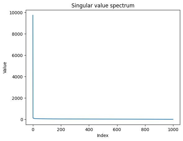
We reduce the researcher–paper matrix to its top-k singular components to capture the most important interaction patterns. Then we provide a simple lookup function that fetches the predicted score for any researcher–paper pair from this compressed representation.
def opt_rank_k_approximation(m: np.ndarray, k: int):
    """Returns the optimal rank-k reconstruction matrix, using SVD."""

    assert 0 < k <= np.min(m.shape), f"The rank must be in [0, min(m, n)]"

    U, S, Vh = np.linalg.svd(m, full_matrices=False)

    U_k = U[:, :k]
    S_k = S[:k]
    Vh_k = Vh[:k]

    return np.dot(U_k * S_k, Vh_k)


def matrix_pred_fn(train_recon: np.ndarray, sids: np.ndarray, pids: np.ndarray) -> np.ndarray:
    """
    Input:
        train_recon: (M, N) matrix with predicted values for every (sid, pid) pair.
        sids: (D,) vector with integer scientist IDs.
        pids: (D,) vector with integer paper IDs.

    Outputs: (D,) vector with predictions.
    """

    return train_recon[sids, pids]
We compute a rank-2 low-rank approximation of the training matrix via SVD by calling opt_rank_k_approximation(train_mat, k=2).
train_recon = opt_rank_k_approximation(train_mat, k=2)
pred_fn = lambda sids, pids: matrix_pred_fn(train_recon, sids, pids)

# Evaluate on validation data
val_score = evaluate(valid_ratings_df, pred_fn)
print(f"Validation RMSE: {val_score:.3f}")
Validation RMSE: 1.186
Method 2: Learned embeddings
| Next, we will take a machine learning view of the problem. To each scientist and paper, we assign a \(d\)-dimensional embedding and we predict the rating that the scientist gives the paper to be their dot product. More formally, let \(\vec{s}_i\) be a scientist embedding and \(\vec{p}_j\) be a paper embedding. Then, we make the following rating prediction for this pair: \(\tilde{r}_{ij} = \langle \vec{s}_i, \vec{p}_j \rangle.\) We view these embeddings as our learnable parameters and train them as we would any other model using the squared error loss function: \(\ell(\theta) = \frac{1}{2}\) | \(\langle \vec{s}_i, \vec{p}_j \rangle - r_{ij}^2\) | Note: \(\theta = \{ \vec{s}_i \}_{i=1}^n \cup \{ \vec{p}_j \}_{j=1}^m\). The following is an implementation of this method. |
class EmbeddingDotProductModel(nn.Module):
    def __init__(self, num_scientists: int, num_papers: int, dim: int):
        super().__init__()

        # Assign to each scientist and paper an embedding
        self.scientist_emb = nn.Embedding(num_scientists, dim)
        self.paper_emb = nn.Embedding(num_papers, dim)

    def forward(self, sid: torch.Tensor, pid: torch.Tensor) -> torch.Tensor:
        """
        Inputs:
            sid: [B,], int
            pid: [B,], int

        Outputs: [B,], float
        """

        # Per-pair dot product
        return torch.sum(self.scientist_emb(sid) * self.paper_emb(pid), dim=-1)
# Define model (10k scientists, 1k papers, 32-dimensional embeddings) and optimizer
model = EmbeddingDotProductModel(10_000, 1_000, 64).to(device)
optim = torch.optim.AdamW(model.parameters(), lr=1e-3, weight_decay=1e-5)
We convert the Pandas DataFrames into PyTorch TensorDatasets containing researcher IDs, paper IDs, and ratings for easy batching.
We then create DataLoaders with batch size 64—shuffled for training and sequential for validation—to feed data into our models.
def get_dataset(df: pd.DataFrame):
    sids = torch.tensor(df["sid"].values, dtype=torch.long)
    pids = torch.tensor(df["pid"].values, dtype=torch.long)
    ratings = torch.tensor(df["rating"].values, dtype=torch.float32)
    return torch.utils.data.TensorDataset(sids, pids, ratings)

train_dataset = get_dataset(train_ratings_df)
valid_dataset = get_dataset(valid_ratings_df)

train_loader = torch.utils.data.DataLoader(train_dataset, batch_size=64, shuffle=True)
valid_loader = torch.utils.data.DataLoader(valid_dataset, batch_size=64, shuffle=False)
We train the model for \(5\) epochs over researcher–paper batches, minimizing MSE and updating parameters via backpropagation, but the training loss isn’t improving substantially.
We’ll need to explore other more advanced techniques to boost performance.
NUM_EPOCHS = 5
for epoch in range(NUM_EPOCHS):
    model.train()
    total_loss, total_count = 0.0, 0
    for sid, pid, ratings in train_loader:
        sid = sid.to(device)
        pid = pid.to(device)
        ratings = ratings.to(device)

        preds = model(sid, pid)
        loss = F.mse_loss(preds, ratings)

        optim.zero_grad()
        loss.backward()
        optim.step()

        total_loss += loss.item() * len(sid)
        total_count += len(sid)

    print(f"[Epoch {epoch+1}/{NUM_EPOCHS}] Train Loss: {total_loss / total_count:.4f}")
[Epoch 1/5] Train Loss: 53.4843
[Epoch 2/5] Train Loss: 19.9365
[Epoch 3/5] Train Loss: 3.3771
[Epoch 4/5] Train Loss: 1.2094
[Epoch 5/5] Train Loss: 0.9402
pred_fn = lambda sids, pids: model(torch.from_numpy(sids).to(device), torch.from_numpy(pids).to(device))

# Evaluate on validation data
with torch.no_grad():
    val_score = evaluate(valid_ratings_df, pred_fn)

print(f"Validation RMSE: {val_score:.3f}")
Validation RMSE: 1.042
Method 3: Iterative SVD Imputation
We start with the incomplete researcher–paper matrix (M), fill missing entries with initial estimates to get (M^{(0)}), and then repeat:
Compute truncated SVD on the current matrix: \(M^{(t-1)} = U\,\Sigma\,V^T, \qquad M_k^{(t)} = U_k\,\Sigma_k\,V_k^T\)
Update only the missing entries: \(M^{(t)}_{ij} = \begin{cases} M_{ij}, & \text{if }(i,j)\text{ observed},\\ \bigl(M_k^{(t)}\bigr)_{ij}, & \text{if }(i,j)\text{ missing}. \end{cases}\)
Measure change on the missing entries: \(\Delta^{(t)} = \bigl\|\,\bigl(M_k^{(t)}\bigr)_{\text{missing}} \;-\; M^{(t-1)}_{\text{missing}} \bigr\|_2\)
We stop when (\Delta^{(t)}) falls below the tolerance, and then use the final matrix (M^{(*)}) to score researcher–paper pairs by simple indexing.
def iterative_svd(df, k=2, max_iterations=10, tolerance=0.001):
    mat = read_data_matrix(df)
    missing_mask = np.isnan(mat)
    imputed_mat = impute_values(mat)

    for iteration in range(max_iterations):
        previous_mat = imputed_mat.copy()
        reconstructed_mat = opt_rank_k_approximation(imputed_mat, k)

        imputed_mat = mat.copy()
        imputed_mat[missing_mask] = reconstructed_mat[missing_mask]

        diff = np.linalg.norm(reconstructed_mat[missing_mask] - previous_mat[missing_mask])
        print(f"Iteration {iteration + 1}, Change: {diff:.6f}")

        if diff < tolerance:
            print(f"Converged after {iteration + 1} iterations")
            break

    return imputed_mat
We choose \(k=2\) to capture the two most significant latent factors, set max_iterations=200 for sufficient refinement, and use a tolerance of \(10^{-4}\) to ensure stable convergence.
final_mat = iterative_svd(train_ratings_df, k=2, max_iterations=200, tolerance=0.0001)
Iteration 1, Change: 358.604161
Iteration 2, Change: 281.641703
Iteration 3, Change: 229.566501
Iteration 4, Change: 192.320822
Iteration 5, Change: 164.490904
Iteration 6, Change: 142.951880
Iteration 7, Change: 125.801054
Iteration 8, Change: 111.826364
Iteration 9, Change: 100.224236
Iteration 10, Change: 90.442575
Iteration 11, Change: 82.089858
Iteration 12, Change: 74.880570
Iteration 13, Change: 68.601350
Iteration 14, Change: 63.089309
Iteration 15, Change: 58.217755
Iteration 16, Change: 53.886528
Iteration 17, Change: 50.015309
Iteration 18, Change: 46.538876
Iteration 19, Change: 43.403681
Iteration 20, Change: 40.565323
Iteration 21, Change: 37.986667
Iteration 22, Change: 35.636408
Iteration 23, Change: 33.487973
Iteration 24, Change: 31.518657
Iteration 25, Change: 29.708947
Iteration 26, Change: 28.041987
Iteration 27, Change: 26.503140
Iteration 28, Change: 25.079641
Iteration 29, Change: 23.760309
Iteration 30, Change: 22.535311
Iteration 31, Change: 21.395969
Iteration 32, Change: 20.334598
Iteration 33, Change: 19.344366
Iteration 34, Change: 18.419185
Iteration 35, Change: 17.553613
Iteration 36, Change: 16.742769
Iteration 37, Change: 15.982267
Iteration 38, Change: 15.268155
Iteration 39, Change: 14.596862
Iteration 40, Change: 13.965154
Iteration 41, Change: 13.370100
Iteration 42, Change: 12.809030
Iteration 43, Change: 12.279514
Iteration 44, Change: 11.779334
Iteration 45, Change: 11.306461
Iteration 46, Change: 10.859035
Iteration 47, Change: 10.435351
Iteration 48, Change: 10.033840
Iteration 49, Change: 9.653060
Iteration 50, Change: 9.291679
Iteration 51, Change: 8.948469
Iteration 52, Change: 8.622295
Iteration 53, Change: 8.312104
Iteration 54, Change: 8.016924
Iteration 55, Change: 7.735850
Iteration 56, Change: 7.468043
Iteration 57, Change: 7.212724
Iteration 58, Change: 6.969164
Iteration 59, Change: 6.736689
Iteration 60, Change: 6.514667
Iteration 61, Change: 6.302509
Iteration 62, Change: 6.099666
Iteration 63, Change: 5.905624
Iteration 64, Change: 5.719903
Iteration 65, Change: 5.542051
Iteration 66, Change: 5.371649
Iteration 67, Change: 5.208300
Iteration 68, Change: 5.051635
Iteration 69, Change: 4.901305
Iteration 70, Change: 4.756984
Iteration 71, Change: 4.618366
Iteration 72, Change: 4.485162
Iteration 73, Change: 4.357100
Iteration 74, Change: 4.233927
Iteration 75, Change: 4.115401
Iteration 76, Change: 4.001296
Iteration 77, Change: 3.891399
Iteration 78, Change: 3.785510
Iteration 79, Change: 3.683437
Iteration 80, Change: 3.585004
Iteration 81, Change: 3.490040
Iteration 82, Change: 3.398386
Iteration 83, Change: 3.309892
Iteration 84, Change: 3.224415
Iteration 85, Change: 3.141821
Iteration 86, Change: 3.061982
Iteration 87, Change: 2.984777
Iteration 88, Change: 2.910093
Iteration 89, Change: 2.837822
Iteration 90, Change: 2.767861
Iteration 91, Change: 2.700113
Iteration 92, Change: 2.634487
Iteration 93, Change: 2.570894
Iteration 94, Change: 2.509252
Iteration 95, Change: 2.449482
Iteration 96, Change: 2.391511
Iteration 97, Change: 2.335266
Iteration 98, Change: 2.280680
Iteration 99, Change: 2.227689
Iteration 100, Change: 2.176233
Iteration 101, Change: 2.126253
Iteration 102, Change: 2.077693
Iteration 103, Change: 2.030502
Iteration 104, Change: 1.984628
Iteration 105, Change: 1.940024
Iteration 106, Change: 1.896645
Iteration 107, Change: 1.854447
Iteration 108, Change: 1.813388
Iteration 109, Change: 1.773429
Iteration 110, Change: 1.734531
Iteration 111, Change: 1.696659
Iteration 112, Change: 1.659777
Iteration 113, Change: 1.623854
Iteration 114, Change: 1.588856
Iteration 115, Change: 1.554754
Iteration 116, Change: 1.521518
Iteration 117, Change: 1.489121
Iteration 118, Change: 1.457536
Iteration 119, Change: 1.426737
Iteration 120, Change: 1.396700
Iteration 121, Change: 1.367401
Iteration 122, Change: 1.338817
Iteration 123, Change: 1.310928
Iteration 124, Change: 1.283711
Iteration 125, Change: 1.257146
Iteration 126, Change: 1.231216
Iteration 127, Change: 1.205900
Iteration 128, Change: 1.181181
Iteration 129, Change: 1.157041
Iteration 130, Change: 1.133465
Iteration 131, Change: 1.110436
Iteration 132, Change: 1.087939
Iteration 133, Change: 1.065959
Iteration 134, Change: 1.044481
Iteration 135, Change: 1.023492
Iteration 136, Change: 1.002978
Iteration 137, Change: 0.982927
Iteration 138, Change: 0.963326
Iteration 139, Change: 0.944163
Iteration 140, Change: 0.925426
Iteration 141, Change: 0.907105
Iteration 142, Change: 0.889188
Iteration 143, Change: 0.871664
Iteration 144, Change: 0.854525
Iteration 145, Change: 0.837759
Iteration 146, Change: 0.821358
Iteration 147, Change: 0.805312
Iteration 148, Change: 0.789612
Iteration 149, Change: 0.774249
Iteration 150, Change: 0.759215
Iteration 151, Change: 0.744503
Iteration 152, Change: 0.730103
Iteration 153, Change: 0.716009
Iteration 154, Change: 0.702213
Iteration 155, Change: 0.688708
Iteration 156, Change: 0.675486
Iteration 157, Change: 0.662541
Iteration 158, Change: 0.649867
Iteration 159, Change: 0.637457
Iteration 160, Change: 0.625304
Iteration 161, Change: 0.613403
Iteration 162, Change: 0.601748
Iteration 163, Change: 0.590333
Iteration 164, Change: 0.579152
Iteration 165, Change: 0.568201
Iteration 166, Change: 0.557473
Iteration 167, Change: 0.546964
Iteration 168, Change: 0.536669
Iteration 169, Change: 0.526583
Iteration 170, Change: 0.516701
Iteration 171, Change: 0.507018
Iteration 172, Change: 0.497531
Iteration 173, Change: 0.488234
Iteration 174, Change: 0.479124
Iteration 175, Change: 0.470196
Iteration 176, Change: 0.461447
Iteration 177, Change: 0.452872
Iteration 178, Change: 0.444467
Iteration 179, Change: 0.436229
Iteration 180, Change: 0.428155
Iteration 181, Change: 0.420240
Iteration 182, Change: 0.412482
Iteration 183, Change: 0.404876
Iteration 184, Change: 0.397420
Iteration 185, Change: 0.390110
Iteration 186, Change: 0.382943
Iteration 187, Change: 0.375917
Iteration 188, Change: 0.369027
Iteration 189, Change: 0.362272
Iteration 190, Change: 0.355648
Iteration 191, Change: 0.349153
Iteration 192, Change: 0.342784
Iteration 193, Change: 0.336538
Iteration 194, Change: 0.330413
Iteration 195, Change: 0.324406
Iteration 196, Change: 0.318515
Iteration 197, Change: 0.312737
Iteration 198, Change: 0.307070
Iteration 199, Change: 0.301512
Iteration 200, Change: 0.296060
pred_iter_svd = lambda sids, pids: matrix_pred_fn(final_mat, sids, pids).flatten()

val_score = evaluate(valid_ratings_df, pred_iter_svd)
print(f"Validation RMSE: {val_score:.3f}")
Validation RMSE: 0.875
The validation performance is just enough to pass the simple baseline, so we will now explore advanced neural methods like NeuMF, DMF, or hybrid combinations of both to improve recommendation accuracy.
Method 4: SVD++
We extend basic matrix factorization by adding user/item biases and modeling implicit feedback. Each researcher \(r\) and paper \(p\) has embeddings \(\mathbf{p}_r,\mathbf{q}_p\in\mathbb{R}^d\), biases \(b_r,b_p\in\mathbb{R}\), and implicit-feedback embeddings \(\{y_j\}\). We predict
\[\hat r_{rp} = \mu + b_r + b_p + \mathbf{q}_p^T\Bigl(\mathbf{p}_r + \frac{1}{\sqrt{|\mathcal{N}(r)|}}\sum_{j\in\mathcal{N}(r)} y_j\Bigr),\]where \(\mu\) is the global mean and \(\mathcal{N}(r)\) is the set of papers researcher \(r\) has interacted with. We train all parameters by minimizing the squared error loss
\[\ell(\theta) = \frac12\bigl(\hat r_{rp} - r_{rp}\bigr)^2.\]class SVDPP(nn.Module):
def __init__(self, num_users, num_items, emb_dim=32):
super().__init__()
self.user_emb = nn.Embedding(num_users, emb_dim)
self.item_emb = nn.Embedding(num_items, emb_dim)
self.user_bias = nn.Embedding(num_users, 1)
self.item_bias = nn.Embedding(num_items, 1)
self.implicit_emb = nn.Embedding(num_items + 1, emb_dim, padding_idx=num_items) # Padding index = num_items
self.global_mean = nn.Parameter(torch.tensor(3.0), requires_grad=False)
def forward(self, user_ids, item_ids, implicit_items):
p_u = self.user_emb(user_ids)
q_i = self.item_emb(item_ids)
b_u = self.user_bias(user_ids).squeeze()
b_i = self.item_bias(item_ids).squeeze()
mask = (implicit_items != self.implicit_emb.padding_idx).unsqueeze(-1)
y_j = self.implicit_emb(implicit_items) * mask
norm = torch.sqrt(mask.sum(dim=1).clamp(min=1).float())
implicit_sum = y_j.sum(dim=1) / norm
x_u = p_u + implicit_sum
dot = (x_u * q_i).sum(dim=1)
return self.global_mean + b_u + b_i + dot
We instantiate the SVD++ model for \(10\,000\) researchers and \(1\,000\) papers, each represented in a \(16\)-dimensional embedding space to capture diverse latent factors.
The Adam optimizer is configured with a learning rate of \(10^{-3}\) and an L2 weight decay of \(10^{-4}\) to balance rapid learning with regularization.
A ReduceLROnPlateau scheduler monitors the validation loss and, if it does not improve for one epoch, halves the learning rate to allow finer-grained updates and more stable convergence.
model_svdpp = SVDPP(num_users=10_000, num_items=1_000, emb_dim=16).to(device)
optim_svdpp = torch.optim.Adam(model_svdpp.parameters(), lr=1e-3, weight_decay=1e-4)
scheduler = torch.optim.lr_scheduler.ReduceLROnPlateau(optim_svdpp, mode='min', factor=0.5, patience=1)
We create a fixed-size implicit-feedback matrix where each of the 10 000 researchers is assigned a list of up to 50 papers they have interacted with.
Using a defaultdict, we first collect all paper IDs for each researcher. We then build a NumPy array of shape (10 000, 50), filling unused slots with a padding index equal to the number of items.
Finally, we convert this array into a PyTorch tensor on the target device so it can be fed directly into the SVD++ model as implicit feedback.
from collections import defaultdict

def build_implicit_item_matrix(df, num_users, num_items, max_len=50):
    PAD_IDX = num_items
    user_implicit = defaultdict(list)
    for _, row in df.iterrows():
        user_implicit[int(row['sid'])].append(int(row['pid']))
    matrix = np.full((num_users, max_len), fill_value=PAD_IDX, dtype=int)
    for user_id, items in user_implicit.items():
        matrix[user_id, :min(len(items), max_len)] = items[:max_len]
    return torch.tensor(matrix, dtype=torch.long)

NUM_USERS = 10_000
NUM_ITEMS = 1_000
EMB_DIM = 16
MAX_LEN = 50

implicit_matrix = build_implicit_item_matrix(train_ratings_df, NUM_USERS, NUM_ITEMS, max_len=MAX_LEN).to(device)
Over 10 epochs, we alternate between training and validation.
During training, for each batch of researcher–paper pairs we mask out the current paper from the researcher’s implicit list, predict ratings with SVD++, compute MSE loss, and update parameters via Adam.
In validation, we again mask the held‐out paper, compute predictions without gradient updates, and aggregate the squared errors to report RMSE.
A ReduceLROnPlateau scheduler adjusts the learning rate based on the validation loss for more stable convergence.
# Cell 4: Training and Validation Loop with Masking Current Item and RMSE Logging
NUM_EPOCHS = 10
PAD_IDX = model_svdpp.implicit_emb.padding_idx

for epoch in range(NUM_EPOCHS):
    model_svdpp.train()
    train_loss_total, train_count = 0.0, 0
    for sid, pid, ratings in train_loader:
        sid = sid.to(device)
        pid = pid.to(device)
        ratings = ratings.to(device)

        # clone and mask out current item from implicit feedback
        imp_items = implicit_matrix[sid].clone()
        imp_items[imp_items == pid.unsqueeze(1)] = PAD_IDX

        preds = model_svdpp(sid, pid, imp_items)
        loss = F.mse_loss(preds, ratings)

        optim_svdpp.zero_grad()
        loss.backward()
        optim_svdpp.step()

        train_loss_total += loss.item() * sid.size(0)
        train_count += sid.size(0)

    avg_train_loss = train_loss_total / train_count

    model_svdpp.eval()
    val_mse_total, val_count = 0.0, 0
    with torch.no_grad():
        for sid, pid, ratings in valid_loader:
            sid = sid.to(device)
            pid = pid.to(device)
            ratings = ratings.to(device)

            imp_items = implicit_matrix[sid].clone()
            imp_items[imp_items == pid.unsqueeze(1)] = PAD_IDX

            preds = model_svdpp(sid, pid, imp_items)
            mse = F.mse_loss(preds, ratings, reduction='sum')

            val_mse_total += mse.item()
            val_count += sid.size(0)

    valid_rmse = (val_mse_total / val_count) ** 0.5
    print(f"Epoch {epoch + 1}/{NUM_EPOCHS} – Train Loss: {avg_train_loss:.4f}, Valid RMSE: {valid_rmse:.4f}")
    scheduler.step(val_mse_total / val_count)
Epoch 1/10 – Train Loss: 9.9278, Valid RMSE: 1.3532
Epoch 2/10 – Train Loss: 1.0362, Valid RMSE: 0.9103
Epoch 3/10 – Train Loss: 0.7914, Valid RMSE: 0.8869
Epoch 4/10 – Train Loss: 0.7730, Valid RMSE: 0.8815
Epoch 5/10 – Train Loss: 0.7670, Valid RMSE: 0.8799
Epoch 6/10 – Train Loss: 0.7639, Valid RMSE: 0.8788
Epoch 7/10 – Train Loss: 0.7626, Valid RMSE: 0.8787
Epoch 8/10 – Train Loss: 0.7610, Valid RMSE: 0.8788
Epoch 9/10 – Train Loss: 0.7602, Valid RMSE: 0.8778
Epoch 10/10 – Train Loss: 0.7595, Valid RMSE: 0.8782
pred_fn_svdpp = lambda sids, pids: model_svdpp(
    torch.from_numpy(sids).to(device),
    torch.from_numpy(pids).to(device),
    implicit_matrix[
        torch.from_numpy(np.clip(sids, 0, implicit_matrix.shape[0] - 1)).to(device)
    ]
).detach().cpu().numpy()

with torch.no_grad():
    val_score = evaluate(valid_ratings_df, pred_fn_svdpp)

print(f"Validation RMSE: {val_score:.3f}")
Validation RMSE: 0.878
After training, we achieved a validation RMSE of 0.878, which again only just beats our simple baseline.
However, SVD++ allowed extensive hyperparameter tuning—embedding size, learning rate, weight decay, and scheduler settings—and the current configuration represents the best combination we found. This fine-tuning flexibility, along with the model’s ability to incorporate both biases and implicit feedback, makes SVD++ preferable to the more rigid iterative SVD approach. Additional advantages include faster convergence on sparse data and a straightforward path to extend with dropout or deeper bias structures if needed.
Note: Wishlist Data Incorporation
From this point, we incorporate the wishlist information by passing both the ratings DataFrame (with columns sid, pid, rating) and the wishlist DataFrame (with columns sid, pid) into get_dataset. Inside the function, we first tag every wishlist entry with wishlist = 1.0 and then perform a full outer join on (sid, pid), ensuring that any researcher–paper pair present in either list appears exactly once. After merging, we fill missing rating or wishlist values with 0.0 (indicating no explicit rating or no wishlist flag), convert each column into a PyTorch tensor, and pack them into a TensorDataset of (sid, pid, rating, wishlist_flag) for downstream training.
def get_dataset(
    df: pd.DataFrame,
    wishlist_df: pd.DataFrame = None
) -> torch.utils.data.Dataset:
    """
    Returns a dataset of (sid, pid, rating, wishlist_flag) for every
    (sid,pid) in ratings OR wishlist.  Missing ratings or wishlist
    entries are filled with 0.0.
    """
    # If no wishlist provided, just add an empty wishlist column
    if wishlist_df is None:
        merged = df.copy()
        merged['wishlist'] = 0.0

    else:
        w = wishlist_df[['sid', 'pid']].copy()
        w['wishlist'] = 1.0

        merged = pd.merge(
            df[['sid', 'pid', 'rating']],
            w,
            on=['sid', 'pid'],
            how='outer'       # <-- full join
        )

        merged['rating'] = merged['rating'].fillna(0.0)
        merged['wishlist'] = merged['wishlist'].fillna(0.0)

    sids      = torch.from_numpy(merged['sid'].to_numpy()).long()
    pids      = torch.from_numpy(merged['pid'].to_numpy()).long()
    ratings   = torch.from_numpy(merged['rating'].to_numpy()).float()
    wishlists = torch.from_numpy(merged['wishlist'].to_numpy()).float()

    return torch.utils.data.TensorDataset(sids, pids, ratings, wishlists)
Method 5: Neural Matrix Factorization (NeuMF)
We build a hybrid model that learns both linear and nonlinear interactions and jointly predicts ratings and wishlist preferences. NeuMF combines a GMF branch (element-wise product of embeddings) with an MLP branch (deep concatenation of embeddings), fuses them via a learned weight \(\alpha\), and uses separate output heads for rating and wishlist signals.
Detailed Architecture
Input embeddings
Each researcher \(r\) and paper \(p\) has a \(d\)-dimensional embedding \(\mathbf{u}_r,\mathbf{v}_p\in\mathbb{R}^d\).GMF branch
\(g = \mathbf{u}_r \odot \mathbf{v}_p\)MLP branch
Concatenate and feed through hidden layers:
\(x^{(1)} = [\mathbf{u}_r, \mathbf{v}_p],\quad x^{(\ell+1)} = \mathrm{GELU}(W^{(\ell)} x^{(\ell)} + b^{(\ell)}),\;\ell=1,\dots,L\) yielding \(m = x^{(L+1)}\).Fusion
\(f = [\,\alpha\,g,\;(1-\alpha)\,m\,],\quad \alpha\in[0,1]\ \text{learned}\)- Output heads
- Rating:
\(\hat r = 1 + 4\;\sigma\bigl(W_r\,f + b_r\bigr),\)
constraining \(\hat r\in[1,5]\). - Wishlist:
\(\hat w = \sigma\bigl(W_w\,f + b_w\bigr),\quad \hat w\in[0,1].\)
- Rating:
- Loss function
Combine rating MSE (only where no wishlist) and wishlist MSE:
\(\ell = \frac{1}{2}\|\hat r - r\|^2_{\!(w=0)} \;+\;\lambda\,\|\hat w - w\|^2,\)
where \(\|\cdot\|_{(w=0)}\) masks out entries with \(w=1\), and \(\lambda\) is the wishlist weight.
This design lets NeuMF capture both simple latent-factor signals and high-order nonlinear interactions, simultaneously optimizing for two complementary tasks.
class GMF(nn.Module):
    def __init__(self, num_researchers, num_papers, emb_dim):
        super().__init__()
        self.researcher_emb = nn.Embedding(num_researchers, emb_dim)
        self.paper_emb = nn.Embedding(num_papers, emb_dim)
        self.dropout = nn.Dropout(0.2)

    def forward(self, researcher_indices, paper_indices):
        r = self.dropout(self.researcher_emb(researcher_indices))
        p = self.dropout(self.paper_emb(paper_indices))
        return r * p

class MLP(nn.Module):
    def __init__(self, num_researchers, num_papers, emb_dim, mlp_layers):
        super().__init__()
        self.researcher_emb = nn.Embedding(num_researchers, emb_dim)
        self.paper_emb = nn.Embedding(num_papers, emb_dim)
        self.dropout = nn.Dropout(0.2)
        layers = []
        input_size = emb_dim * 2
        for h in mlp_layers:
            layers += [nn.Linear(input_size, h), nn.GELU(), nn.Dropout(0.2)]
            input_size = h
        self.mlp = nn.Sequential(*layers)

    def forward(self, researcher_indices, paper_indices):
        r = self.dropout(self.researcher_emb(researcher_indices))
        p = self.dropout(self.paper_emb(paper_indices))
        x = torch.cat([r, p], dim=1)
        return self.mlp(x)

class NeuMF(nn.Module):
    def __init__(self, num_researchers, num_papers, emb_dim, mlp_layers, wishlist_weight=2.0):
        super().__init__()
        self.gmf = GMF(num_researchers, num_papers, emb_dim)
        self.mlp = MLP(num_researchers, num_papers, emb_dim, mlp_layers)
        self.alpha = nn.Parameter(torch.tensor(0.5))
        self.wishlist_weight = wishlist_weight

        final_size = emb_dim + mlp_layers[-1]
        self.fc_rating = nn.Linear(final_size, 1)
        self.fc_wishlist = nn.Linear(final_size, 1)

    def forward(self, researcher_indices, paper_indices):
        g = self.gmf(researcher_indices, paper_indices)
        m = self.mlp(researcher_indices, paper_indices)
        fused = torch.cat([self.alpha * g, (1 - self.alpha) * m], dim=1)
        rating = 1 + 4 * torch.sigmoid(self.fc_rating(fused).squeeze(1))
        wishlist = torch.sigmoid(self.fc_wishlist(fused).squeeze(1))
        return rating, wishlist

    def calc_loss(self, rating_pred, rating_target, wishlist_pred, wishlist_target):
        # Only compute rating loss where wishlist_target is 0
        mask = wishlist_target == 0
        rating_loss = F.mse_loss(rating_pred[mask], rating_target[mask])
        wishlist_loss = F.mse_loss(wishlist_pred, wishlist_target)
        return rating_loss + self.wishlist_weight * wishlist_loss
train_dataset = get_dataset(train_ratings_df, train_wishlist_df)
valid_dataset = get_dataset(valid_ratings_df)

train_loader = torch.utils.data.DataLoader(train_dataset, batch_size=64, shuffle=True)
valid_loader = torch.utils.data.DataLoader(valid_dataset, batch_size=64, shuffle=False)
We configure the NeuMF model with \(10,000\) researchers and \(1,000\) papers, embedding each into a \(16\)-dimensional latent space and using two MLP hidden layers of size \(32\).
The wishlist loss is weighted by \(2.0\), and training runs for \(40\) epochs with batch size \(64\), using AdamW at learning rate \(5\times10^{-3}\) and L2 regularization; a ReduceLROnPlateau scheduler halves the learning rate if validation loss does not improve for one epoch.
NUM_USERS = 10_000
NUM_ITEMS = 1_000
EMB_DIM = 16
MLP_HIDDEN = [32, 32]
WISHLIST_LOSS_WEIGHT = 2.0
BATCH_SIZE = 64
NUM_EPOCHS = 40
LEARNING_RATE = 5e-3

model_neumf = NeuMF(NUM_USERS, NUM_ITEMS, EMB_DIM, MLP_HIDDEN, WISHLIST_LOSS_WEIGHT).to(device)
optimizer = torch.optim.AdamW(model_neumf.parameters(), lr=LEARNING_RATE)
scheduler = torch.optim.lr_scheduler.ReduceLROnPlateau(optimizer, mode='min', factor=0.5, patience=1)
The NeuMF training loop mirrors the SVD++ procedure: over \(40\) epochs we perform forward/backward passes with AdamW on each batch’s ratings and wishlist flags, then compute validation RMSE (clamping ratings to \([1,5]\)) and step the ReduceLROnPlateau scheduler.
NUM_EPOCHS = 40
for epoch in range(NUM_EPOCHS):
    model_neumf.train()
    running_loss = 0.0

    for sid, pid, ratings, wishlists in train_loader:
        sid, pid = sid.to(device), pid.to(device)
        ratings, wishlists = ratings.to(device), wishlists.to(device)

        pred_ratings, pred_wishlist = model_neumf(sid, pid)
        loss = model_neumf.calc_loss(pred_ratings, ratings, pred_wishlist, wishlists)

        optimizer.zero_grad()
        loss.backward()
        optimizer.step()

        running_loss += loss.item() * sid.size(0)

    avg_train_loss = running_loss / len(train_loader.dataset)

    # Validation
    model_neumf.eval()
    mse_total = 0.0
    with torch.no_grad():
        for sid, pid, ratings, _ in valid_loader:
            sid, pid = sid.to(device), pid.to(device)
            ratings = ratings.to(device)

            pred_ratings, _ = model_neumf(sid, pid)
            mse = F.mse_loss(pred_ratings.clamp(1, 5), ratings)
            mse_total += mse.item() * sid.size(0)

    rmse = (mse_total / len(valid_loader.dataset)) ** 0.5
    print(f"Epoch {epoch + 1}/{NUM_EPOCHS} – Train Loss: {avg_train_loss:.4f}, Valid RMSE: {rmse:.4f}")
    scheduler.step(rmse)
Epoch 1/40 – Train Loss: 1.2049, Valid RMSE: 0.9039
Epoch 2/40 – Train Loss: 1.1356, Valid RMSE: 0.9056
Epoch 3/40 – Train Loss: 1.1269, Valid RMSE: 0.8964
Epoch 4/40 – Train Loss: 1.1112, Valid RMSE: 0.8905
Epoch 5/40 – Train Loss: 1.0988, Valid RMSE: 0.8889
Epoch 6/40 – Train Loss: 1.0920, Valid RMSE: 0.8867
Epoch 7/40 – Train Loss: 1.0842, Valid RMSE: 0.8854
Epoch 8/40 – Train Loss: 1.0792, Valid RMSE: 0.8851
Epoch 9/40 – Train Loss: 1.0761, Valid RMSE: 0.8812
Epoch 10/40 – Train Loss: 1.0736, Valid RMSE: 0.8848
Epoch 11/40 – Train Loss: 1.0736, Valid RMSE: 0.8797
Epoch 12/40 – Train Loss: 1.0719, Valid RMSE: 0.8822
Epoch 13/40 – Train Loss: 1.0705, Valid RMSE: 0.8792
Epoch 14/40 – Train Loss: 1.0701, Valid RMSE: 0.8748
Epoch 15/40 – Train Loss: 1.0704, Valid RMSE: 0.8779
Epoch 16/40 – Train Loss: 1.0691, Valid RMSE: 0.8768
Epoch 17/40 – Train Loss: 1.0231, Valid RMSE: 0.8610
Epoch 18/40 – Train Loss: 1.0144, Valid RMSE: 0.8617
Epoch 19/40 – Train Loss: 1.0161, Valid RMSE: 0.8620
Epoch 20/40 – Train Loss: 0.9803, Valid RMSE: 0.8534
Epoch 21/40 – Train Loss: 0.9721, Valid RMSE: 0.8543
Epoch 22/40 – Train Loss: 0.9718, Valid RMSE: 0.8532
Epoch 23/40 – Train Loss: 0.9734, Valid RMSE: 0.8553
Epoch 24/40 – Train Loss: 0.9743, Valid RMSE: 0.8536
Epoch 25/40 – Train Loss: 0.9470, Valid RMSE: 0.8499
Epoch 26/40 – Train Loss: 0.9398, Valid RMSE: 0.8499
Epoch 27/40 – Train Loss: 0.9389, Valid RMSE: 0.8493
Epoch 28/40 – Train Loss: 0.9392, Valid RMSE: 0.8507
Epoch 29/40 – Train Loss: 0.9398, Valid RMSE: 0.8504
Epoch 30/40 – Train Loss: 0.9213, Valid RMSE: 0.8491
Epoch 31/40 – Train Loss: 0.9174, Valid RMSE: 0.8486
Epoch 32/40 – Train Loss: 0.9168, Valid RMSE: 0.8490
Epoch 33/40 – Train Loss: 0.9162, Valid RMSE: 0.8486
Epoch 34/40 – Train Loss: 0.9050, Valid RMSE: 0.8485
Epoch 35/40 – Train Loss: 0.9028, Valid RMSE: 0.8485
Epoch 36/40 – Train Loss: 0.9015, Valid RMSE: 0.8487
Epoch 37/40 – Train Loss: 0.8954, Valid RMSE: 0.8485
Epoch 38/40 – Train Loss: 0.8941, Valid RMSE: 0.8486
Epoch 39/40 – Train Loss: 0.8919, Valid RMSE: 0.8485
Epoch 40/40 – Train Loss: 0.8907, Valid RMSE: 0.8484
os.makedirs("models", exist_ok=True)
torch.save(model_neumf.state_dict(), "models/neumf.pt")
print("Model saved to models/neumf.pt")
Model saved to models/neumf.pt
pred_fn_neumf = lambda sids, pids: model_neumf(
    torch.from_numpy(sids).to(device),
    torch.from_numpy(pids).to(device)
)[0].clamp(1, 5).detach().cpu().numpy()

# Evaluate on validation data
with torch.no_grad():
    val_score = evaluate(valid_ratings_df, pred_fn_neumf)

print(f"Validation RMSE: {val_score:.3f}")
Validation RMSE: 0.848
The NeuMF model outperformed our previous baselines—marking the first time we beat the hard benchmark—with surprisingly strong validation results.
Achieving this required extensive tuning: we set the wishlist loss weight to \(2.0\) (since MSE is less severe than binary cross-entropy, allowing a coefficient higher than 1), kept embedding and hidden layer sizes modest to prevent overfitting, and applied a relatively high weight decay \(\lambda\) for regularization. Too large a decay would prevent the model from learning (training loss wouldn’t decrease), so this configuration yielded the best overall performance.
Method 6: Graph-Augmented NeuMF (GraphNeuMF)
We model researcher–paper interactions as a bipartite graph to propagate information across similar nodes. Let (A) be the adjacency matrix and (\tilde D) its degree matrix; LightGCN refines initial embeddings (X^{(0)}) via
\[X^{(l+1)} = \tilde D^{-1}A\,X^{(l)},\qquad l = 0,\dots,L-1,\]and aggregates them into
\[X = \frac{1}{L+1}\sum_{l=0}^L X^{(l)}.\]After pretraining with a BPR loss to separate positive and negative edges, we extract the user and paper rows of (X) and fuse them with GMF’s elementwise product and MLP’s encoding into a combined vector (f). Two output heads then compute:
Rating
\(\hat r = 1 + 4\,\sigma\bigl(W_r f + b_r\bigr),\)Wishlist
\(\hat w = \sigma\bigl(W_w f + b_w\bigr).\)
We train both tasks with mean-squared error, weighting the wishlist term by (\lambda_{\text{wish}}):
\[\ell = \mathrm{MSE}(\hat r, r) \;+\; \lambda_{\text{wish}}\;\mathrm{MSE}(\hat w, w).\]class LightGCN(nn.Module):
def __init__(self, num_users, num_items, emb_dim, num_layers=3):
super().__init__()
self.num_users = num_users
self.num_items = num_items
self.emb_dim = emb_dim
self.num_layers = num_layers
self.user_emb = nn.Embedding(num_users, emb_dim)
self.item_emb = nn.Embedding(num_items, emb_dim)
nn.init.xavier_uniform_(self.user_emb.weight)
nn.init.xavier_uniform_(self.item_emb.weight)
# graph convolution layers
from torch_geometric.nn import LGConv
self.convs = nn.ModuleList([
LGConv(normalize=True) for _ in range(num_layers)
])
# will hold a SparseTensor
self.adj = None
def set_adj(self, edge_index: torch.LongTensor, device: torch.device):
# build and store the adjacency once
self.adj = SparseTensor(
row=edge_index[0],
col=edge_index[1] + self.num_users,
sparse_sizes=(self.num_users + self.num_items,) * 2
).to(device)
def forward(self):
x = torch.cat([self.user_emb.weight, self.item_emb.weight], dim=0)
embeddings = [x]
for conv in self.convs:
x = conv(x, self.adj)
embeddings.append(x)
x = torch.mean(torch.stack(embeddings), dim=0)
user_emb, item_emb = torch.split(x, [self.num_users, self.num_items])
return user_emb, item_emb
def get_embeddings(self, user_idx, item_idx):
return self.user_emb(user_idx), self.item_emb(item_idx)
class GraphNeuMF(nn.Module):
def __init__(self, num_users, num_items, emb_dim, mlp_layers, wishlist_weight):
super().__init__()
self.lightgcn = LightGCN(num_users, num_items, emb_dim)
self.gmf = GMF(num_users, num_items, emb_dim)
self.mlp = MLP(num_users, num_items, emb_dim, mlp_layers)
self.alpha = nn.Parameter(torch.tensor(0.5))
self.wishlist_weight = wishlist_weight
final_size = emb_dim + mlp_layers[-1] + emb_dim + emb_dim
self.fc_rating = nn.Linear(final_size, 1)
self.fc_wishlist = nn.Linear(final_size, 1)
def forward(self, user_idx, item_idx):
user_emb_g, item_emb_g = self.lightgcn.get_embeddings(user_idx, item_idx)
gmf_out = self.gmf(user_idx, item_idx)
mlp_out = self.mlp(user_idx, item_idx)
fused = torch.cat([
self.alpha * gmf_out,
(1.0 - self.alpha) * mlp_out,
user_emb_g,
item_emb_g
], dim=1)
fused = fused if fused.dim() > 1 else fused.unsqueeze(0)
rating_pred = 1.0 + 4.0 * torch.sigmoid(self.fc_rating(fused).squeeze(1))
wishlist_prob = torch.sigmoid(self.fc_wishlist(fused).squeeze(1))
return rating_pred, wishlist_prob
def calc_loss(self, rating_pred, rating_target, wishlist_pred, wishlist_target):
mask_r = (wishlist_target == 0.0)
rating_loss = F.mse_loss(rating_pred[mask_r], rating_target[mask_r])
wishlist_loss = F.mse_loss(wishlist_pred, wishlist_target)
return rating_loss + self.wishlist_weight * wishlist_loss
This constructs a bipartite edge list by stacking researcher and paper indices—optionally filtering to only wishlist interactions—into a 2×E tensor (edge_index) for graph-based models.
def build_interaction_graph_from_dataset(
    dataset: torch.utils.data.TensorDataset,
    use_wishlist: bool = True
) -> torch.LongTensor:
    sids, pids, ratings, wishlists = dataset.tensors
    if use_wishlist:
        mask = wishlists == 1.0
    else:
        mask = torch.ones_like(wishlists, dtype=torch.bool)

    edge_index = torch.stack([sids[mask], pids[mask]], dim=0)
    return edge_index
train_dataset = get_dataset(train_ratings_df, train_wishlist_df)
valid_dataset = get_dataset(valid_ratings_df)

edge_index = build_interaction_graph_from_dataset(train_dataset, use_wishlist=False).to(device)

train_loader = torch.utils.data.DataLoader(train_dataset, batch_size=BATCH_SIZE, shuffle=True)
valid_loader = torch.utils.data.DataLoader(valid_dataset, batch_size=BATCH_SIZE, shuffle=False)
We configure GraphNeuMF with \(10,000\) researchers and \(1,000\) papers, embedding each into a \(16\)-dimensional space and using two MLP hidden layers of size 32.
The wishlist loss weight is set to 2.0 (as with NeuMf where we have fined-tunned this hyperparameter), batch size to 64, and learning rate to \(10^{-3}\).
Before joint training, we precompute and set the LightGCN adjacency (edge_index) to enable efficient graph convolutions.
NUM_USERS       = 10_000
NUM_ITEMS       = 1_000
EMB_DIM         = 16
MLP_LAYERS      = [32, 32]
WISHLIST_WEIGHT = 2.0
BATCH_SIZE      = 64
LEARNING_RATE   = 1e-3

model_graphneumf = GraphNeuMF(
    num_users=NUM_USERS,
    num_items=NUM_ITEMS,
    emb_dim=EMB_DIM,
    mlp_layers=MLP_LAYERS,
    wishlist_weight=2.0
).to(device)

# precompute adjacency
model_graphneumf.lightgcn.set_adj(edge_index, device)
We pretrain the LightGCN layers for \(5\) epochs using a BPR-style loss that encourages higher scores for observed researcher–paper edges than for randomly sampled negatives. This step refines the graph-based embeddings before they are fused into the GraphNeuMF model.
print("Pre-training LightGCN...")
pretrain_opt       = torch.optim.Adam(model_graphneumf.lightgcn.parameters(), lr=0.01)
GCN_PRETRAIN_EPOCHS= 5

for epoch in range(GCN_PRETRAIN_EPOCHS):
    model_graphneumf.lightgcn.train()
    pretrain_opt.zero_grad()

    user_emb, item_emb = model_graphneumf.lightgcn()
    pos_u, pos_i       = edge_index
    neg_i              = torch.randint(0, NUM_ITEMS, (edge_index.size(1)*10,), device=device)

    pos_scores = (user_emb[pos_u] * item_emb[pos_i]).sum(dim=1)
    neg_scores = (user_emb[pos_u.repeat(10)] * item_emb[neg_i]).sum(dim=1)

    loss = -torch.log(torch.sigmoid(pos_scores.repeat(10) - neg_scores)).mean()
    loss.backward()
    pretrain_opt.step()

    print(f" Pre-train Epoch {epoch+1}/{GCN_PRETRAIN_EPOCHS}  Loss={loss.item():.4f}")
    if loss.item() < 0.5:
        break
Pre-training LightGCN...
 Pre-train Epoch 1/5  Loss=0.6931
 Pre-train Epoch 2/5  Loss=0.6931
 Pre-train Epoch 3/5  Loss=0.6931
 Pre-train Epoch 4/5  Loss=0.6931
 Pre-train Epoch 5/5  Loss=0.6931
The GraphNeuMF training loop is almost identical to NeuMF’s: over \(40\) epochs we batch researcher–paper pairs (and wishlist flags), compute the combined rating and wishlist loss, backpropagate with AdamW, and step a ReduceLROnPlateau scheduler based on validation RMSE.
This end-to-end training fine-tunes both the graph-based embeddings and the hybrid NeuMF components together, yielding the final GraphNeuMF model.
optimizer = torch.optim.AdamW(model_graphneumf.parameters(), lr=LEARNING_RATE)
scheduler = torch.optim.lr_scheduler.ReduceLROnPlateau(
    optimizer, mode='min', factor=0.5, patience=1
)
NUM_EPOCHS = 40
for epoch in range(1, NUM_EPOCHS+1):
    model_graphneumf.train()
    tot_loss, tot_n = 0.0, 0

    for sid, pid, ratings, wishlists in train_loader:
        sid, pid = sid.to(device), pid.to(device)
        ratings, wishlists = ratings.to(device), wishlists.to(device)

        pr, pw = model_graphneumf(sid, pid)
        loss   = model_graphneumf.calc_loss(pr, ratings, pw, wishlists)

        optimizer.zero_grad()
        loss.backward()
        optimizer.step()

        tot_loss += loss.item() * sid.size(0)
        tot_n    += sid.size(0)

    avg_train_loss = tot_loss / tot_n

    # validation
    model_graphneumf.eval()
    val_mse, val_n = 0.0, 0
    with torch.no_grad():
        for sid, pid, ratings, _ in valid_loader:
            sid, pid   = sid.to(device), pid.to(device)
            ratings    = ratings.to(device)
            pred_r, _  = model_graphneumf(sid, pid)
            pred_r_cl  = pred_r.clamp(1.0, 5.0)
            val_mse   += F.mse_loss(pred_r_cl, ratings, reduction='sum').item()
            val_n     += sid.size(0)

    valid_rmse = (val_mse / val_n) ** 0.5
    print(f"[Epoch {epoch}/{NUM_EPOCHS}] "
          f"Train loss={avg_train_loss:.4f}, Valid RMSE={valid_rmse:.4f}")

    scheduler.step(valid_rmse)
[Epoch 1/40] Train loss=1.1383, Valid RMSE=0.9000
[Epoch 2/40] Train loss=1.0966, Valid RMSE=0.8970
[Epoch 3/40] Train loss=1.0899, Valid RMSE=0.8969
[Epoch 4/40] Train loss=1.0821, Valid RMSE=0.8969
[Epoch 5/40] Train loss=1.0704, Valid RMSE=0.8965
[Epoch 6/40] Train loss=1.0524, Valid RMSE=0.8931
[Epoch 7/40] Train loss=1.0249, Valid RMSE=0.8857
[Epoch 8/40] Train loss=1.0001, Valid RMSE=0.8788
[Epoch 9/40] Train loss=0.9861, Valid RMSE=0.8733
[Epoch 10/40] Train loss=0.9767, Valid RMSE=0.8699
[Epoch 11/40] Train loss=0.9688, Valid RMSE=0.8669
[Epoch 12/40] Train loss=0.9642, Valid RMSE=0.8644
[Epoch 13/40] Train loss=0.9592, Valid RMSE=0.8619
[Epoch 14/40] Train loss=0.9571, Valid RMSE=0.8609
[Epoch 15/40] Train loss=0.9532, Valid RMSE=0.8597
[Epoch 16/40] Train loss=0.9505, Valid RMSE=0.8580
[Epoch 17/40] Train loss=0.9483, Valid RMSE=0.8580
[Epoch 18/40] Train loss=0.9463, Valid RMSE=0.8569
[Epoch 19/40] Train loss=0.9446, Valid RMSE=0.8567
[Epoch 20/40] Train loss=0.9430, Valid RMSE=0.8572
[Epoch 21/40] Train loss=0.9419, Valid RMSE=0.8558
[Epoch 22/40] Train loss=0.9413, Valid RMSE=0.8555
[Epoch 23/40] Train loss=0.9393, Valid RMSE=0.8561
[Epoch 24/40] Train loss=0.9380, Valid RMSE=0.8558
[Epoch 25/40] Train loss=0.9078, Valid RMSE=0.8527
[Epoch 26/40] Train loss=0.9010, Valid RMSE=0.8528
[Epoch 27/40] Train loss=0.8993, Valid RMSE=0.8532
[Epoch 28/40] Train loss=0.8805, Valid RMSE=0.8529
[Epoch 29/40] Train loss=0.8763, Valid RMSE=0.8529
[Epoch 30/40] Train loss=0.8657, Valid RMSE=0.8528
[Epoch 31/40] Train loss=0.8635, Valid RMSE=0.8528
[Epoch 32/40] Train loss=0.8569, Valid RMSE=0.8530
[Epoch 33/40] Train loss=0.8569, Valid RMSE=0.8529
[Epoch 34/40] Train loss=0.8530, Valid RMSE=0.8530
[Epoch 35/40] Train loss=0.8520, Valid RMSE=0.8532
[Epoch 36/40] Train loss=0.8505, Valid RMSE=0.8531
[Epoch 37/40] Train loss=0.8507, Valid RMSE=0.8531
[Epoch 38/40] Train loss=0.8501, Valid RMSE=0.8530
[Epoch 39/40] Train loss=0.8494, Valid RMSE=0.8530
[Epoch 40/40] Train loss=0.8487, Valid RMSE=0.8529
pred_fn_graphneumf = lambda sids, pids: model_graphneumf(
    torch.from_numpy(sids).to(device),
    torch.from_numpy(pids).to(device)
)[0].clamp(1, 5).detach().cpu().numpy()

# Evaluate on validation data
with torch.no_grad():
    val_score = evaluate(valid_ratings_df, pred_fn_graphneumf)

print(f"Validation RMSE: {val_score:.3f}")
Validation RMSE: 0.853
Although GraphNeuMF did not improve on the validation RMSE of \(0.848\) achieved by NeuMF alone, its longer training schedule limited our ability to fine-tune its hyperparameters.
We anticipate that GraphNeuMF explores complementary regions of the embedding space compared to NeuMF, making their combination in a future ensemble potentially more powerful.
Method 6: Deep Matrix Factorization (DMF)
Deep Matrix Factorization (DMF) replaces shallow embeddings with two “towers” of nonlinear transformations, one for researchers and one for papers. Each tower maps initial embeddings into a deep latent space, and predictions are made by combining these deep representations.
Specifically, let
\(\mathbf{e}_r \in \mathbb{R}^d,\quad \mathbf{e}_p \in \mathbb{R}^d\)
be the researcher and paper embeddings. We apply \(L\) layers of transformations:
\(\mathbf{u} = f_r(\mathbf{e}_r),\quad \mathbf{v} = f_p(\mathbf{e}_p),\)
where each \(f(\cdot)\) is a sequence of linear + GELU blocks. The predicted rating is
\(\hat r_{rp} = \mathbf{u}^\top \mathbf{v} \;+\; b_r \;+\; b_p \;+\; \beta,\)
with researcher bias \(b_r\), paper bias \(b_p\), and global bias \(\beta\). Implicit feedback is modeled via a BPR loss on wishlist logits, and the overall objective combines MSE on observed ratings with weighted BPR plus embedding regularization:
\(\mathcal{L} = \mathrm{MSE}(\hat r, r) \;+\;\lambda_\text{wish}\,\mathrm{BPR}(\ell^+, \ell^-) \;+\;\lambda_\text{emb}\|\mathbf{e}\|_2^2.\)
def make_block(in_f, out_f):
    return nn.Sequential(
        nn.Linear(in_f, out_f),
        nn.GELU(),
    )

class DMF(nn.Module):
    def __init__(
        self,
        num_users,
        num_items,
        layers,
        wishlist_weight=0.5,
        max_rating=5.0,
        embed_lambda=1e-5,
    ):
        super().__init__()
        self.max_rating           = max_rating
        self.wishlist_weight = wishlist_weight
        self.embed_lambda         = embed_lambda

        emb_dim = layers[0]
        self.u_emb       = nn.Embedding(num_users, emb_dim)
        self.i_emb       = nn.Embedding(num_items, emb_dim)
        self.u_bias      = nn.Embedding(num_users, 1)
        self.i_bias      = nn.Embedding(num_items, 1)
        self.global_bias = nn.Parameter(torch.zeros(1))

        self.dropout = nn.Dropout(0.2)

        self.user_tower = nn.Sequential(*[
            make_block(layers[i], layers[i+1])
            for i in range(len(layers) - 1)
        ])
        self.item_tower = nn.Sequential(*[
            make_block(layers[i], layers[i+1])
            for i in range(len(layers) - 1)
        ])

        self.fc_wish = nn.Linear(layers[-1], 1)

    @staticmethod
    def bpr_loss(pos_score, neg_score):
        return -F.logsigmoid(pos_score - neg_score).mean()

    def forward(self, u_idx, i_idx):
        u = self.dropout(self.u_emb(u_idx))
        v = self.dropout(self.i_emb(i_idx))

        u = self.user_tower(u)
        v = self.item_tower(v)

        x = u * v

        dot    = x.sum(dim=1)
        ub     = self.u_bias(u_idx).squeeze(1)
        ib     = self.i_bias(i_idx).squeeze(1)
        rating = dot + ub + ib + self.global_bias

        wish_logit = self.fc_wish(x).squeeze(1)
        wish       = torch.sigmoid(wish_logit)

        return rating, wish, wish_logit

    def calc_loss(
        self,
        rating_pred,
        rating_true,
        wish_logit_pos=None,
        wish_logit_neg=None,
    ):
        mask = rating_true > 0
        rating_loss = F.mse_loss(rating_pred[mask], rating_true[mask])

        if wish_logit_pos is None or wish_logit_neg is None:
            imp_loss = torch.tensor(0., device=rating_pred.device, dtype=rating_pred.dtype)
        else:
            imp_loss = self.bpr_loss(wish_logit_pos, wish_logit_neg)

        base = rating_loss + self.wishlist_weight * imp_loss

        emb_reg = (
            self.u_emb.weight.norm(p=2).pow(2)
          + self.i_emb.weight.norm(p=2).pow(2)
        ) * self.embed_lambda

        return base + 0.5 * emb_reg
train_dataset = get_dataset(train_ratings_df, train_wishlist_df)
valid_dataset = get_dataset(valid_ratings_df)

train_loader = torch.utils.data.DataLoader(train_dataset, batch_size=64, shuffle=True)
valid_loader = torch.utils.data.DataLoader(valid_dataset, batch_size=64, shuffle=False)
We initialize DMF for \(10{,}000\) researchers and \(1{,}000\) papers with tower layer sizes \([32,64,128]\), embedding dimension \(32\) (which is the first tower dim), and a wishlist weight of \(0.5\).
The AdamW optimizer uses a learning rate of \(10^{-3}\), weight decay of \(10^{-3}\), and embedding regularization \(\lambda_{\text{emb}}=10^{-4}\).
A ReduceLROnPlateau scheduler halves the learning rate if validation RMSE does not improve for one epoch.
NUM_USERS   = 10000
NUM_ITEMS   = 1000
MLP_HIDDEN  = [32, 64, 128]
LEARNING_RATE = 1e-3
WEIGHT_DECAY  = 1e-3
EMBED_LAMBDA  = 1e-4

device = torch.device('cuda' if torch.cuda.is_available() else 'cpu')
model_dmf = DMF(NUM_USERS, NUM_ITEMS, MLP_HIDDEN, wishlist_weight=0.5, max_rating=5.0, embed_lambda=EMBED_LAMBDA).to(device)
optimizer = torch.optim.AdamW(model_dmf.parameters(), lr=LEARNING_RATE, weight_decay=WEIGHT_DECAY)
scheduler = torch.optim.lr_scheduler.ReduceLROnPlateau(optimizer, mode='min', factor=0.5, patience=1)
The DMF training loop follows the same pattern as NeuMF and GraphNeuMF—batch-wise forward/backward passes with AdamW and ReduceLROnPlateau—while additionally performing BPR-style negative sampling: for each positive wishlist example we sample a random negative paper and compute a pairwise loss \(\ell_{\text{BPR}} = -\log\sigma(s^+ - s^-)\) to encourage higher scores for true interactions.
NUM_EPOCHS = 40
for epoch in range(NUM_EPOCHS):
    model_dmf.train()
    running_loss = 0.0

    for sid, pid, ratings, wishlists in train_loader:
        sid, pid   = sid.to(device), pid.to(device)
        ratings    = ratings.to(device)
        wishlists  = wishlists.to(device)

        pred_ratings, _, wish_logit = model_dmf(sid, pid)

        # BPR negative sampling using wishlist flag
        pos_idx = (wishlists > 0).nonzero(as_tuple=True)[0]
        if pos_idx.numel() > 0:
            pos_scores = wish_logit[pos_idx]
            u_pos      = sid[pos_idx]
            neg_items  = torch.randint(0, NUM_ITEMS, (pos_idx.size(0),), device=device)
            _, _, neg_logits = model_dmf(u_pos, neg_items)
        else:
            pos_scores, neg_logits = None, None

        loss = model_dmf.calc_loss(
            pred_ratings, ratings,
            pos_scores, neg_logits
        )

        optimizer.zero_grad()
        loss.backward()
        optimizer.step()
        running_loss += loss.item() * sid.size(0)

    avg_train_loss = running_loss / len(train_loader.dataset)

    model_dmf.eval()
    mse_sum = 0.0
    with torch.no_grad():
        for sid, pid, ratings, _ in valid_loader:
            sid, pid   = sid.to(device), pid.to(device)
            ratings    = ratings.to(device)
            pred_ratings, _, _ = model_dmf(sid, pid)
            pred_ratings       = pred_ratings.clamp(1, model_dmf.max_rating)
            mse_sum += F.mse_loss(pred_ratings, ratings, reduction='sum').item()

    rmse = (mse_sum / len(valid_loader.dataset)) ** 0.5
    print(f"Epoch {epoch+1}/{NUM_EPOCHS} – Train Loss: {avg_train_loss:.4f}, Valid RMSE: {rmse:.4f}")
    scheduler.step(rmse)
Epoch 1/40 – Train Loss: 3.5817, Valid RMSE: 0.9294
Epoch 2/40 – Train Loss: 1.2795, Valid RMSE: 0.9193
Epoch 3/40 – Train Loss: 1.1961, Valid RMSE: 0.9053
Epoch 4/40 – Train Loss: 1.1603, Valid RMSE: 0.8953
Epoch 5/40 – Train Loss: 1.1356, Valid RMSE: 0.8904
Epoch 6/40 – Train Loss: 1.1162, Valid RMSE: 0.8825
Epoch 7/40 – Train Loss: 1.0984, Valid RMSE: 0.8771
Epoch 8/40 – Train Loss: 1.0862, Valid RMSE: 0.8760
Epoch 9/40 – Train Loss: 1.0817, Valid RMSE: 0.8732
Epoch 10/40 – Train Loss: 1.0798, Valid RMSE: 0.8746
Epoch 11/40 – Train Loss: 1.0786, Valid RMSE: 0.8732
Epoch 12/40 – Train Loss: 1.0408, Valid RMSE: 0.8611
Epoch 13/40 – Train Loss: 1.0272, Valid RMSE: 0.8594
Epoch 14/40 – Train Loss: 1.0246, Valid RMSE: 0.8575
Epoch 15/40 – Train Loss: 1.0219, Valid RMSE: 0.8560
Epoch 16/40 – Train Loss: 1.0200, Valid RMSE: 0.8555
Epoch 17/40 – Train Loss: 1.0186, Valid RMSE: 0.8551
Epoch 18/40 – Train Loss: 1.0176, Valid RMSE: 0.8534
Epoch 19/40 – Train Loss: 1.0150, Valid RMSE: 0.8536
Epoch 20/40 – Train Loss: 1.0143, Valid RMSE: 0.8531
Epoch 21/40 – Train Loss: 1.0122, Valid RMSE: 0.8535
Epoch 22/40 – Train Loss: 1.0121, Valid RMSE: 0.8522
Epoch 23/40 – Train Loss: 1.0106, Valid RMSE: 0.8517
Epoch 24/40 – Train Loss: 1.0090, Valid RMSE: 0.8510
Epoch 25/40 – Train Loss: 1.0085, Valid RMSE: 0.8502
Epoch 26/40 – Train Loss: 1.0078, Valid RMSE: 0.8498
Epoch 27/40 – Train Loss: 1.0072, Valid RMSE: 0.8490
Epoch 28/40 – Train Loss: 1.0065, Valid RMSE: 0.8488
Epoch 29/40 – Train Loss: 1.0057, Valid RMSE: 0.8493
Epoch 30/40 – Train Loss: 1.0040, Valid RMSE: 0.8491
Epoch 31/40 – Train Loss: 0.9642, Valid RMSE: 0.8439
Epoch 32/40 – Train Loss: 0.9492, Valid RMSE: 0.8439
Epoch 33/40 – Train Loss: 0.9446, Valid RMSE: 0.8436
Epoch 34/40 – Train Loss: 0.9418, Valid RMSE: 0.8441
Epoch 35/40 – Train Loss: 0.9405, Valid RMSE: 0.8438
Epoch 36/40 – Train Loss: 0.9117, Valid RMSE: 0.8438
Epoch 37/40 – Train Loss: 0.9023, Valid RMSE: 0.8438
Epoch 38/40 – Train Loss: 0.8828, Valid RMSE: 0.8455
Epoch 39/40 – Train Loss: 0.8788, Valid RMSE: 0.8454
Epoch 40/40 – Train Loss: 0.8652, Valid RMSE: 0.8466
pred_fn_dmf = lambda sids, pids: (
    model_dmf(
        torch.from_numpy(sids).long().to(device),
        torch.from_numpy(pids).long().to(device)
    )[0].detach().cpu().numpy()
)

# Evaluate on validation data
with torch.no_grad():
    val_score = evaluate(valid_ratings_df, pred_fn_dmf)

print(f"Validation RMSE: {val_score:.3f}")
Validation RMSE: 0.847
The DMF model reaches validation RMSE comparable to NeuMF but trains much faster, making it well-suited for quick experimentation. We switched to a combined MSE + BPR objective—\(\ell_{\text{BPR}} = -\log\sigma(s^+ - s^-)\)—to better leverage implicit wishlist signals, and added a global bias term \(\beta\) to center our predictions.
To prevent overfitting, we increased the embedding regularization to \(\lambda_{\text{emb}}=10^{-4}\) and applied a weight decay of \(10^{-3}\) across all parameters. The deep tower architecture ([32, 64, 128]) provides greater representational power, while these regularization settings ensure the model generalizes effectively.
All the hyperparameters were greatly fined-tuned for the best performance!
Put it all together: Ensamble
We gather our four base predictors—NeuMF, DMF, SVD++, and GraphNeuMF—into a dictionary for easy access, and extract the true ratings from the training and validation sets to serve as targets for ensemble weighting.
This setup allows us to experiment with various blending strategies (simple average, weighted average, stacking) by evaluating each predictor’s outputs against true_ratings_valid.
prediction_functions = {
    "NeuMF": pred_fn_neumf,
    "DMF": pred_fn_dmf,
    "SVD++": pred_fn_svdpp,
    "GraphNeuMF": pred_fn_graphneumf,
}

true_ratings_train = train_ratings_df["rating"].values
true_ratings_valid = valid_ratings_df["rating"].values
def get_model_predictions(df, model_name):
    sids, pids = df["sid"].values, df["pid"].values
    return prediction_functions[model_name](sids, pids)

train_predictions = {name: get_model_predictions(train_ratings_df, name) for name in prediction_functions}
valid_predictions = {name: get_model_predictions(valid_ratings_df, name) for name in prediction_functions}
Get each model raw performance
base_model_rmses = {
    name: np.sqrt(np.mean((valid_predictions[name] - true_ratings_valid) ** 2))
    for name in prediction_functions
}

for name, rmse in base_model_rmses.items():
    print(f"{name} Validation RMSE: {rmse:.4f}")

best_base_model = min(base_model_rmses, key=base_model_rmses.get)
best_base_rmse = base_model_rmses[best_base_model]
NeuMF Validation RMSE: 0.8484
DMF Validation RMSE: 0.8475
SVD++ Validation RMSE: 0.8782
GraphNeuMF Validation RMSE: 0.8519
For simple averaging, we compute
\(\hat r_i \;=\; \frac{1}{M}\sum_{m=1}^M \hat r_i^{(m)}\)
and report its RMSE.
For weighted averaging, we define
\(w_m \;=\; \frac{1/\mathrm{RMSE}_m}{\sum_{j=1}^M (1/\mathrm{RMSE}_j)}, \quad \hat r_i \;=\; \sum_{m=1}^M w_m\,\hat r_i^{(m)}\)
so that more accurate models carry greater influence, and then compute the resulting RMSE.
# Simple Average
avg_preds = np.mean(list(valid_predictions.values()), axis=0)
avg_rmse = np.sqrt(np.mean((avg_preds - true_ratings_valid) ** 2))
print(f"Simple Average RMSE: {avg_rmse:.4f}")

# Weighted Average
inv_rmses = {k: 1/v for k, v in base_model_rmses.items()}
norm = sum(inv_rmses.values())
weights = {k: v / norm for k, v in inv_rmses.items()}

weighted_preds = sum(weights[k] * valid_predictions[k] for k in weights)
weighted_rmse = np.sqrt(np.mean((weighted_preds - true_ratings_valid) ** 2))
print(f"Weighted Average RMSE: {weighted_rmse:.4f}")
Simple Average RMSE: 0.8371
Weighted Average RMSE: 0.8370
We construct meta-features for each example by stacking the two base predictions and their average and difference into
\(\mathbf{x}_i = \bigl[\hat r_i^{(1)},\;\hat r_i^{(2)},\;\tfrac{\hat r_i^{(1)}+\hat r_i^{(2)}}{2},\;\hat r_i^{(1)}-\hat r_i^{(2)}\bigr]^\top,\)
then standardize each feature to zero mean and unit variance.
A small DeepStacking neural network maps \(\mathbf{x}'_i\mapsto\hat r_i\) through one hidden layer of size \(4\times dim\) and a final output neuron, training to minimize
\(\mathcal{L} = \frac{1}{N}\sum_{i=1}^N\bigl(\hat r_i - r_i\bigr)^2.\)
from sklearn.preprocessing import StandardScaler

def create_meta_features(pred_dict):
    preds = list(pred_dict.values())
    return np.vstack([
        preds[0],
        preds[1],
        np.mean(preds, axis=0),
        preds[0] - preds[1]
    ]).T

X_train = create_meta_features(train_predictions)
X_valid = create_meta_features(valid_predictions)

scaler = StandardScaler()
X_train_scaled = scaler.fit_transform(X_train)
X_valid_scaled = scaler.transform(X_valid)

X_train_tensor = torch.tensor(X_train_scaled, dtype=torch.float32).to(device)
X_valid_tensor = torch.tensor(X_valid_scaled, dtype=torch.float32).to(device)
y_train_tensor = torch.tensor(true_ratings_train, dtype=torch.float32).to(device)
y_valid_tensor = torch.tensor(true_ratings_valid, dtype=torch.float32).to(device)
class DeepStacking(nn.Module):
    def __init__(self, in_dim, p_drop=0.2):
        super().__init__()
        h1 = 4 * in_dim
        self.net = nn.Sequential(
            nn.Linear(in_dim, h1),
            nn.BatchNorm1d(h1),
            nn.GELU(),
            nn.Dropout(p_drop),
            nn.Linear(h1, 1),
        )

    def forward(self, x):
        return self.net(x).squeeze(-1)


# model, optimizer, loss
stack_model = DeepStacking(X_train.shape[1]).to(device)
optimizer = torch.optim.AdamW(stack_model.parameters(), lr=1e-3, weight_decay=1e-3)
loss_fn = nn.MSELoss()

# scheduler: reduce LR on plateau of val RMSE
scheduler = torch.optim.lr_scheduler.ReduceLROnPlateau(
    optimizer,
    mode='min',           # we want to minimize RMSE
    factor=0.5,           # LR = LR * factor
    patience=1 ,          # wait 10 epochs before reducing
)
best_rmse = float("inf")

for epoch in range(10000):
    # ——— Training step ———
    stack_model.train()
    optimizer.zero_grad()
    pred = stack_model(X_train_tensor)
    loss = loss_fn(pred, y_train_tensor)
    loss.backward()
    optimizer.step()

    # ——— Every 250 epochs: evaluate both train and val ———
    if epoch % 250 == 0:
        stack_model.eval()
        with torch.no_grad():
            # training RMSE
            train_preds = stack_model(X_train_tensor)
            train_rmse  = torch.sqrt(loss_fn(train_preds, y_train_tensor)).item()

            # validation RMSE (with clamp if desired)
            val_preds = stack_model(X_valid_tensor).clamp(1, 5)
            val_rmse  = torch.sqrt(loss_fn(val_preds, y_valid_tensor)).item()

            print(
                f"Epoch {epoch:4d} | "
                f"Train RMSE: {train_rmse:.4f} | "
                f"Val   RMSE: {val_rmse:.4f}"
            )

            scheduler.step(val_rmse)

            # checkpoint best
            if val_rmse < best_rmse:
                best_rmse = val_rmse
                best_state = stack_model.state_dict()
Epoch    0 | Train RMSE: 3.7671 | Val   RMSE: 2.9919
Epoch  250 | Train RMSE: 1.9367 | Val   RMSE: 1.9380
Epoch  500 | Train RMSE: 1.3347 | Val   RMSE: 1.3447
Epoch  750 | Train RMSE: 1.1224 | Val   RMSE: 1.1728
Epoch 1000 | Train RMSE: 0.9369 | Val   RMSE: 1.0311
Epoch 1250 | Train RMSE: 0.9020 | Val   RMSE: 0.9991
Epoch 1500 | Train RMSE: 0.7822 | Val   RMSE: 0.9174
Epoch 1750 | Train RMSE: 0.7306 | Val   RMSE: 0.8764
Epoch 2000 | Train RMSE: 0.7201 | Val   RMSE: 0.8689
Epoch 2250 | Train RMSE: 0.7189 | Val   RMSE: 0.8669
Epoch 2500 | Train RMSE: 0.7166 | Val   RMSE: 0.8637
Epoch 2750 | Train RMSE: 0.7150 | Val   RMSE: 0.8631
Epoch 3000 | Train RMSE: 0.7144 | Val   RMSE: 0.8622
Epoch 3250 | Train RMSE: 0.7138 | Val   RMSE: 0.8631
Epoch 3500 | Train RMSE: 0.7131 | Val   RMSE: 0.8606
Epoch 3750 | Train RMSE: 0.7126 | Val   RMSE: 0.8601
Epoch 4000 | Train RMSE: 0.7117 | Val   RMSE: 0.8593
Epoch 4250 | Train RMSE: 0.7119 | Val   RMSE: 0.8588
Epoch 4500 | Train RMSE: 0.7202 | Val   RMSE: 0.8655
Epoch 4750 | Train RMSE: 0.7115 | Val   RMSE: 0.8586
Epoch 5000 | Train RMSE: 0.7103 | Val   RMSE: 0.8579
Epoch 5250 | Train RMSE: 0.7111 | Val   RMSE: 0.8592
Epoch 5500 | Train RMSE: 0.7110 | Val   RMSE: 0.8588
Epoch 5750 | Train RMSE: 0.7109 | Val   RMSE: 0.8590
Epoch 6000 | Train RMSE: 0.7104 | Val   RMSE: 0.8588
Epoch 6250 | Train RMSE: 0.7110 | Val   RMSE: 0.8588
Epoch 6500 | Train RMSE: 0.7110 | Val   RMSE: 0.8591
Epoch 6750 | Train RMSE: 0.7109 | Val   RMSE: 0.8591
Epoch 7000 | Train RMSE: 0.7109 | Val   RMSE: 0.8591
Epoch 7250 | Train RMSE: 0.7109 | Val   RMSE: 0.8591
Epoch 7500 | Train RMSE: 0.7109 | Val   RMSE: 0.8592
Epoch 7750 | Train RMSE: 0.7109 | Val   RMSE: 0.8591
Epoch 8000 | Train RMSE: 0.7109 | Val   RMSE: 0.8591
Epoch 8250 | Train RMSE: 0.7109 | Val   RMSE: 0.8591
Epoch 8500 | Train RMSE: 0.7109 | Val   RMSE: 0.8592
Epoch 8750 | Train RMSE: 0.7109 | Val   RMSE: 0.8591
Epoch 9000 | Train RMSE: 0.7109 | Val   RMSE: 0.8592
Epoch 9250 | Train RMSE: 0.7109 | Val   RMSE: 0.8591
Epoch 9500 | Train RMSE: 0.7109 | Val   RMSE: 0.8592
Epoch 9750 | Train RMSE: 0.7109 | Val   RMSE: 0.8592
stack_model.load_state_dict(best_state)
stack_model.eval()
with torch.no_grad():
    final_preds = stack_model(X_valid_tensor).clamp(1, 5).cpu().numpy()
    final_rmse = np.sqrt(np.mean((final_preds - true_ratings_valid) ** 2))

print(f"\nFinal Linear Stacking RMSE: {final_rmse:.4f}")
Final Linear Stacking RMSE: 0.8592
Finally, we rank the base models by their validation RMSE and select the top (k). For those (k) models, we assign weights proportional to the inverse RMSE:
\[w_m = \frac{1/\mathrm{RMSE}_m}{\sum_{j=1}^k (1/\mathrm{RMSE}_j)},\]then compute the ensemble prediction
\[\hat r_i = \sum_{m=1}^k w_m\,\hat r_i^{(m)}.\]By varying (k) from 2 up to the total number of models, we evaluate the RMSE of each top-(k) ensemble and choose the one with the lowest error.
def top_k_ensemble(k=3):

    sorted_models = sorted(base_model_rmses.items(), key=lambda x: x[1])
    top_models = sorted_models[:k]
    top_model_names = [name for name, _ in top_models]

    print(f"Selected top {k} models: {', '.join(top_model_names)}")


    weights = {}
    sum_weights = sum(1/ rmse for _, rmse in top_models)
    for name, rmse in top_models:
        weights[name] = (1 / rmse) / sum_weights
        print(f"  {name} weight: {weights[name]:.4f}")

    preds = np.zeros_like(true_ratings_valid, dtype=float)
    for name in top_model_names:
        preds += weights[name] * valid_predictions[name]

    rmse = np.sqrt(np.mean((preds - true_ratings_valid) ** 2))
    return preds, rmse, weights, top_model_names
best_k = 0
best_rmse = float('inf')

for k in range(2, len(prediction_functions) + 1):
    _, rmse, _, _ = top_k_ensemble(k)
    if rmse < best_rmse:
        best_rmse = rmse
        best_k = k

print(f"Best Top-{best_k} Ensemble RMSE: {best_rmse:.6f}")
Selected top 2 models: DMF, NeuMF
  DMF weight: 0.5003
  NeuMF weight: 0.4997
Selected top 3 models: DMF, NeuMF, GraphNeuMF
  DMF weight: 0.3340
  NeuMF weight: 0.3337
  GraphNeuMF weight: 0.3323
Selected top 4 models: DMF, NeuMF, GraphNeuMF, SVD++
  DMF weight: 0.2526
  NeuMF weight: 0.2523
  GraphNeuMF weight: 0.2513
  SVD++ weight: 0.2438
Best Top-3 Ensemble RMSE: 0.835264
We found that the optimal ensemble uses the top \(k=3\) models with inverse‐RMSE weights, so we compute the blended predictions accordingly.
Selected top 3 models: DMF, NeuMF, GraphNeuMF
  DMF weight: 0.3340
  NeuMF weight: 0.3337
  GraphNeuMF weight: 0.3323